
Research Methods
Beaver Crossing Historic Research
By Robert Kilts
Introduction
Before railroads became the standard form of heavy freight transportation across the Great Plains, the most common method was the use of freight wagons drawn by ox teams. When the route came to a water barrier such as a river or a creek, the options were limited to bridging or fording. As bridges were a major construction, and timber a limited resource, locating a shallow point with a relatively firm bottom to use for fording was very important. Even with a firm bottom, a gently banking slope was another key feature, since many rivers and creeks cut their banks steeply into the terrain over time. Such a ford required a major effort, especially if the ford was a narrow point passable for only one wagon at a time, when a train of wagons might number fifteen or twenty.
One such crossing of Beaver Creek was found just north of the branch of Beaver Creek from the Blue River. While the bottom was firm, and the banks were relatively gentle, crossing was typically done as the first or the last effort in a day's travel, and naturally, this led to overnight stays being the standard on either the approach side or the departure side.
As with any opportunity for commerce, the numbers of wagons using the trails were at high levels in the early 1860s. Businessmen intending to make profits established facilities on both the east and the west sides of the Beaver Crossing. Their primary customers were travelers on the trail, as well as the sparse population of local homesteaders and farmers.
From 1851 to 1853, James D. Doty led a surveying party through the Great Plains and Rocky Mountains determined to find a suitable route for the future transcontinental railroads, and also to identify the Native American tribes and the territories those tribes controlled. One of his assistants was Amos Reed, son of John Savage Reed, a lawyer in New York state.
Businessmen in Nebraska City, hoping to make it a primary port on the Missouri River, sponsored a survey from Nebraska City to Fort Kearney, attempting to identify a more direct route for westward settlement and freighting. The common route followed the Platte River, which curved around to the north, requiring longer travel times, and higher costs as well as crossing from Council Bluffs, miles to the north. This survey party plotted their route mostly due west. Then they encountered a choice of once more bridging the Blue River or turning north into more rough terrain. Luckily neither was necessary as the ford at Beaver Creek was located. By using the Beaver Crossing, as it came to be known, the route continued into York County, and eventually to Fort Kearney. It was five days travel shorter than the more common route. This Nebraska City Cut-off of the Oregon Trail saw extensive use until railroads became the standard in the early 1870s for long-range heavy transportation.
Once travel was established along the Nebraska City Cut-off, support facilities sprung up almost immediately. Road ranches, where livestock, feed, and supplies could be bought, sold, or traded became common place. There were many road ranches along the Cut-off. The most noted proprietors were Davidson, Thompson, Reed, and Fouse in Seward County, but Reed and Fouse occupied the east and west banks of the Beaver Crossing according to historical records.
Chronology
In 1860 Nebraska City businessmen conducted a survey seeking a more direct route from Nebraska City to Fort Kearney to make freighting business from the Missouri River to Fort Kearney more profitable. A trail following relatively level grade was established the same year, named the Nebraska City Cut-off. Shortly after this, Brigham Young recommended the Cut-off as a replacement starting point for Mormon immigrants, as it saved some five or six days travel time to Fort Kearney. According to Mormon records, more than 6,000 Mormon families used this route from 1861 to 1868.
In 1862, an ambitious project involving trackless steam powered transportation also came to Nebraska City, called the Steam Wagon. The Steam Wagon Road was described as a plowed furrow through the prairie, to mark the proposed route for this project. This project failed as the engine overturned just five miles into its first journey and the inventor was faced with family health issues back in Chicago. Eventually the disabled engine was scavenged for scrap iron.
In 1862, a freight driver named John E. Leonard discussed the news from the east, and decided he would rather not return and join the impending War Between the States. He built a sturdy cabin east of the Beaver Creek ford and raised hay, selling it to passing travelers for a "good price."
In June of 1863, John Fouse bought a cabin and squatter's rights on the west bank of the Beaver Creek ford from a Frenchman named Jean Levigne, where he stocked some general merchandise and contracted as a stage station for the Star Line. According to local histories, Fouse also operated a "Wild West Saloon" at the same location. Local history also claims he had an escape tunnel from his cellar to his dugout stable some 6-8 rods or 60 feet closer to Beaver Creek. His stable was described to have a capacity for six horse teams (12 horses). His son's letter also claims Fouse maintained sufficient black powder in his cellar to "blow up the store" rather than permit it to be captured. He also describes the presence of a dugout stable about 60 feet from the main building, but not the locally legendary tunnel.
In 1866, John Leonard sold his land and cabin to Amos Reed, who had his brother, Roland Reed, and family open a road ranch. The Reed family sold feed and other supplies and traded animals to passing freighters and settlers.
In 1869, Thomas Tisdale came to share the Fouse property, operating a larger general mercantile. While a latecomer, he was responsible for a pivot point in Beaver Crossing history. One of Tisdale's responsibilities was postmaster of the Beaver Crossing post office.
In 1870, the completion of many railroads caused a sharp decline in the traffic along Nebraska wagon routes and a sharp decline in the trail-based businesses located around the Beaver Creek Crossing.
In 1871, Thomas Tisdale closed his store at the ford and relocated to a growing town site some four miles to the east. Rather than change the name of his post office, he simply took the Beaver Crossing name to the new location. Fouse purchased a different property for his primary home, and permitted School District 38 to be formed in his old home. Roland Reed homesteaded with his family east of the new Beaver Crossing location.
Closing out this brief period of intensive business use, Fouse sold his land to relatives named McMichael in the 1880s. Roads and traffic trends to follow the section boundaries left the ford of Beaver Creek as a passing moment in history.
Results from the 2005 Geophysical Investigations at the Beaver Creek Trail Crossing Site (25SW49)
By Arlo McKee
Introduction
During the spring and summer months of 2005, several selected areas of the Beaver Creek Trail Crossing Site were surveyed with various geophysical methods. In advance of the University of Nebraska - Lincoln 2005 summer field school, an initial survey was conducted by Steven De Vore, an archaeologist with the National Park Service, Midwest Archeological Center. The purpose of the initial survey was to investigate the possibility of subsurface archaeological remains in the area of a small mound on the east side of the site. Additionally, the western portion of the site was investigated in an attempt to locate any additional features associated with the set of five trail ruts. The results of this initial survey are summarized in this chapter, but for further information see De Vore (2005).
The second survey took place during the summer field school and fall semester. The purpose of this second survey was two-fold. The eastern portion of the site was examined with metal detectors in an attempt to locate any additional structures on the site. A magnetic survey was conducted over a cluster of metal detector hits in this area. The western portion of the site was also intensively examined with resistance and magnetic instruments. This location was surveyed to determine if the angle at which the initial survey was collected had any effect on the resolution of the historic trail in each dataset. These instruments have been proven to sense historic trail remnants in the past (De Vore 1996; Kvamme 2001). However, as in these studies, the appearance of the trails was simply a side note to other investigations. A precise examination of the resolution of the trails has not been completed and will aid in future subsurface location and mapping of historic trails.
Geophysical Methods
"Archaeology is the one science that destroys its own lab — no repeated experiments . . . it better be done right the first time, or not at all" (Weymouth 1986).The above quote exemplifies the need for good practices in site surveying prior to excavation. Dr. Weymouth of the University of Nebraska–Lincoln physics department was instrumental in developing a standard for geophysical survey in the United States (Weymouth 1986). Geophysical methods for archaeological site surveying have been practiced since the mid 1940s (Clark 1990). Electrical resistivity methods were first practiced in England, where they proved useful, however markedly limited for archaeological purposes. Because of the limited initial success geophysical prospection was slow to gain a commonplace in archaeology. In 1958 the use of the proton magnetometer began to change this situation (Wynn 1986). Compared to resistivity methods, the proton magnetometer allowed for sites to be surveyed relatively quickly. Magnetometers also had the added bonus of being sensitive to fired features such as hearths and kilns. For this reason, magnetometers remain the most commonly used geophysical survey tool. The section below outlines some of the instruments and methods used at the Beaver Crossing Site.
Magnetic Gradient
The magnetic portion of the survey was conducted with the Geoscan Research FM36 fluxgate gradiometer (Geoscan Research 1987:Figure 2.1). The FM36 is capable of a 0.05 nT (nanotesla) resolution and 0.1 nT absolute accuracy. This allows for very subtle changes in the magnetic field of the soil to be sensed (see Bevan 1998; Clark 1990; Kvamme 2001; Milsom 2003; Weymouth 1986 for further information). This instrument measures the earth's magnetic field strength in relation to the position and direction of each sensor. The sensors, thus, must be accurately aligned to the direction of magnetic north at the beginning of each survey day. The gradiometer was carried so that the bottom sensor was located approximately 30 cm above the ground surface. The upper sensor was fixed 50 cm above the bottom. Each sensor reads the magnetic field strength simultaneously at its given position. The gradient magnetic field is calculated by subtracting the top sensor's readings from the bottom. The magnetic gradient is the theoretical magnetic field strength of the soil itself. During each portion of the survey the instrument was set to collect eight readings per meter.
Magnetometers are specifically sensitive to buried ferrous metals. These metals appear in the data as strongly coupled positive and negative values or dipoles. Even a small piece of iron close to the surface can have the effect of overloading the sensors. Care was taken to ensure that the operator of the instrument was completely metal free. Burned soils can also appear in magnetic data if they were heated beyond their Curie point (Gaffney et al. 1991; Kvamme 2001). This process is known as thermoremanent magnetism. The heating of the soil beyond the Curie point causes a reorganization of the atoms. These atoms are newly aligned to point toward magnetic north at the time of heating. This often contrasts with the signature produced by undisturbed soils which generally point toward magnetic north near the time of deposition. Features such as filled ditches can also give anomalous readings because of the relation of iron oxides in the ditch to the fill. Changes in the positions of these elements can create weak magnetic charges in the soil contrast to undisturbed areas (Clark 1990:Figure 2.2). It is because of this property that the historic trails appear weak in magnetic data.
Resistance
The electrical resistance portion of this survey was conducted with the Geoscan RM-15 resistance meter (Geoscan Research 1996:Figure 2.3). This method sends an electric current into the soil via two conducting probes placed a few centimeters in the ground. Two potential probes measure the voltage that is transferred through the ground. The ratio of the voltage to the current that is applied yields the resistance according to Ohm's Law (Weymouth 1986; Clark 1990). (Ohm's law: R=V/I where R=resistance, V=volts, and I=current.) On the RM-15, a pair of current and potential probes is mounted on a mobile frame that is moved around the grid. The two other probes remain fixed in the ground off the survey grid. The mobile are fixed at a 0.5 m separation. This yields an average of 0.75 m depth resolution (Gaffney et al. 1991). The resistance data was collected at 0.5 samples per meter and 1 m between transects.
The principal factor that determines a soil's resistance is its water content and distribution. When the ground is completely saturated, the soil's resistance will be at a minimum because dissolved ions within the soil act as conductors. Buried ditches can appear as areas of lower resistance if they contain more water than the surrounding area. Conversely, worn paths or building foundations have a tendency to repel water and appear as higher resistive areas.
Conductivity
The electrical conductivity portion of the survey was conducted with the Geonics EM38 electromagnetic conductivity meter (Geonics 1992:Figure 2.4) with an Omnidata DL-720 polycorder (Geonics 1998). The EM38 houses two coils, a transmitter and receiver, which are separated 1 m apart. Eddy currents are injected into the ground by the transmitter to a depth roughly equal to the distance between the sensors. The induced magnetic field is then sensed by the receiving coil. In an insulator, the angle between the two components of the electromagnetic field is roughly at 90° (Milsom 2003). Since soils are generally insulators, this is the case and each phase of the field may be measured separately. The EM38 is able to separately measure these two components of the induced field. The in-phase component is a measure of magnetic susceptibility and the out of phase component is the soil conductivity. For this survey, only the out-of-phase field was measured. The conductivity meter was carried so that the transmitting and receiving coils were located as close to the ground as possible. The instrument was set to collect four samples per meter.
Electrical conductivity is the theoretical inverse of resistivity. However, these two instruments collect data in very different ways. Therefore the conductivity meter is sensitive to some features that the resistance meter is not. Buried metals can often react quite strongly to this induced charge. This can cause a signature of extreme values to appear in the data. Another factor affecting the conductivity of the soil is moisture content. The dissolved ions in saturated soil cause a weak conductivity. Disturbed ground, such as ditches and pits, can appear as anomalies in this data as a result of the difference in moisture content with surrounding soils.
Survey Area
The initial geophysical investigation covered two areas within the Beaver Crossing Site (Figure 2.5). One area (location A) was positioned over a small mound on the eastern portion of the site. The area was investigated to confirm the existence of the remains of an 1860s structure. At the start of the survey three 20 m by 20 m grid units were established. The arbitrary grid system was set up parallel to the tree line to the west of the grid. This area was surveyed with magnetic gradient, resistance, conductivity and ground penetrating radar instruments. The second area (location B) was positioned over the series of trail ruts cut into an escarpment. In the area there were also several small depressions that were thought to have a relationship with the trails. Four 20 m by 20 m grid units were established on an arbitrary coordinate system parallel to the escarpment. This area was surveyed with magnetic gradient and conductivity instruments.
The second geophysical investigation expanded the survey area on each side of Beaver Creek. The eastern portion of the site was surveyed with metal detectors to examine the possibility of additional structures in the area (Figure 2.6). The northern lines were laid out roughly 20 m apart and were mapped in using a total station. Based on a cluster of metal detector hits, an additional four 20 m by 20 m grids were magnetically surveyed (location C, Figure 2.7). In order to provide continuity with the initial survey, the same arbitrary coordinate system was used. The final area (location D) was established using the same grid coordinate system as the excavation units and topographic map. This location was positioned over the area surrounding the five trail ruts on the west side of the creek. This coordinate system was advantageous because it allowed for survey transects to be walked nearly perpendicular to the trails. The eastern three grids of location D were magnetically surveyed and the western group of grids was surveyed with magnetic gradient and resistance instruments. There is a small 5 m strip at the top of this area which was not surveyed because of a brush pile.
Field Collection Methods
Under the direction of Steven De Vore, the initial survey locations, A and B, were positioned on the site to avoid any natural obstacles such as trees or ridges. Individual grids were collected using an arbitrary coordinate system with the origin at the southwest corner of each grid. Survey lines marked at intervals of 0.5 m were laid out on the grids to serve as guides for the survey. Each transect was surveyed from east to west with a 1 m separation between transects. The data was then processed and projected into map units for interpretation. Location C was set up using this same arbitrary coordinate system. Location D was set up using the same coordinate system that the test units and topographic map were collected in. This coordinate system was advantageous because it allowed north running transects to be collected nearly perpendicular to the trail ruts. This maximized the number of data points collected along each rut. The data was collected in this way in order to determine if the angle at which the initial survey was collected had any effect on the resolution of the trails. Each magnetometer transect for location D was collected with a 0.5 m separation. In order to conserve time, the resistance survey was collected with 1 m separation between transects.
Data Processing
Because each of the instruments is affected by a number of different ground conditions, it is often necessary to further manipulate the data with post-processing techniques. Although these techniques can enhance the image, an over-application can often result in introducing additional errors in the data. Due to the careful collection in the field, the specific processing techniques that were required remained minimal. A uniform set of processing techniques was used for each of the survey locations.
The magnetic data was first downloaded in the field to GEOPLOT 3.0 (Geoscan Research 2001). The data was then processed with the zero mean traverse function. This function removes inconsistencies in the data due to drift in the sensor during data collection. The data was then interpolated to expand the number of data points to create a 4 x 4 matrix. The arbitrary y-direction which originally contained 8 samples per meter was desampled to fit into the new matrix. This method of interpolation creates a smoother image of the data. A low pass filter was then applied to the data to smooth out the background noise. The magnetic data was then exported into a Golden Software .dat format for processing in Surfer 8 (Golden Software 2002). Finally, a Surfer grid was created using the Krigging method with a 0.25 m cell size. From the Surfer .grd file, both image and 3D plots were made for interpretation.
The resistance data was also downloaded into GEOPLOT 3.0 for processing (Geoscan Research 2001). However, different processing techniques were used. A despike function was first used to remove any false points that the instrument sometimes collects. The despike threshold was set to three standard deviations from the mean. In order to provide continuity between grids, the data was then edge-matched to account for changes in the soil moisture between different days. The data was then interpolated from the original 1 x 2 matrix to a 4 x 4 matrix for a smother image. A low pass filter was also applied to smooth out the background noise. The data was then exported into Surfer as described above.
The conductivity data was initially downloaded into DAT38W software (Geonics 2002). The individual grids were then checked by examining data lines and were exported into the Golden Software .dat format. The resulting grids were then imported into GEOPLOT 3.0 for further processing (Geoscan Research 2001). The data was then processed using a high pass filter. This filter removes low frequency background noise that generally reflects geologic changes in conductivity. To create a smoother image the data was then low pass filtered and interpolated to a 4 x 4 matrix. The data was then exported into Surfer for image generation.
Results
Location A: Under the direction of Steven De Vore, this location was surveyed with magnetic gradient, conductivity, resistance, and ground penetrating radar instruments. The magnetic survey showed a dense cluster of monopole and dipole anomalies in the northern portions of the survey (Figure 2.8). The results from the excavations confirmed that the majority of these anomalies were associated with the metallic remains of an 1860s structure. The conductivity data showed some of the same negative anomalies in the northern portion of the survey (Figure 2.9). The ground penetrating radar data showed the anomaly from the large depression continue to great depth. De Vore noted that this may be the result of a collapsed well (De Vore 2005).
Location B: During the initial survey, location B was also surveyed with magnetic gradient and conductivity instruments. The magnetic survey showed that the area was relatively free from metal anomalies (Figure 2.10). Because of the lack of trash in the area the historic trail ruts appear faintly in the northern portion of the survey. The trail ruts in this data appear as linear anomalies with values near -1 to 1 nT. These values remained consistent with previous studies that included historic trail remnants (Kvamme 2001). The northern-most rut gave the most prominent signal in the magnetic data. The conductivity data similarly shows the trail ruts as slightly higher than average anomalies (Figure 2.11). The several small depressions can also clearly be seen in the conductivity data. These appear as isolated circular positive anomalies. This probably reflects a differential pooling of water in the depressions. The conductivity and magnetic data do not seem to reflect any scatters of metals like location A.
Location C: The east side of Beaver Crossing was surveyed with metal detectors in the hope of locating another structure on site. This survey yielded a number of hits throughout the area (Figure 2.12). Four 20 x 20 m grids were magnetically surveyed to investigate a cluster of strong metal detector hits of consistent depth (Figure 2.13). The bulk of hits were in the southeast portion of the block. A series of dipolar anomalies can be seen in this area that may reflect the same objects that the metal detector sensed. Unlike location A, these anomalies seem to be isolated and may reflect modern trash. It would seem likely that other historic metals could be found in the area, but there does not seem to be any clues pointing toward another building.
Location D: The area containing the five trail remnants was intensively surveyed a second time with magnetic gradient and resistance instruments. This location was ideal for studying trail features because it contains areas where the trails are both visible and invisible on the surface. The area also contains very little trash so that very high resolutions may be obtained from the instruments. The magnetic data clearly displayed the boundaries of the trails on the upper terrace (Figure 2.14). The scarp itself appears as a long linear anomaly that runs southwest to northeast. The northern three trails appear to merge together near the brush pile. The southernmost trail appears to run more southerly in the data. This could be because it is used frequently to enter the lower terrace by the land owner. The eastern group of grids did not contain any anomalies that could be trail features. Overall, this area is very quiet except for two dipolar anomalies. Deposition on the lower floodplain could have resulted in burying the trails too deep to be sensed by the magnetometer. The resistance data also picked up the trails where topography was present (Figure 2.15). However, in the western portion of the survey where the ruts show no local relief they are also invisible to the resistance meter. The data also shows a general trend for the lower flood plain to be generally less resistive than the upper terrace.
Discussion
In order to gain a better understanding of how the trails appeared in each data set, individual profile lines were extracted from the data. This was done using the Surfer grid slice command (Golden Software 2002). Different areas along the trails were examined against the topographic map to identify areas with comparable topography. Over 400 lines of data, cut perpendicular to the trails, were extracted. For comparison, each of the profile lines were centered on the overall mean of the data. Areas with similar topography were horizontally stacked together and averaged to in order to remove unwanted random background noise (Figures 2.16 and 2.17). Generally, the position of the trail appeared to change slightly from one survey to the next. This could be a result of the oblique angle at which the original survey intersected the trail. The relatively few number of data points between transects in the initial survey could have accounted for the trail to appear up to a meter off in one direction. The magnetic profile lines from the initial survey also appear slightly muted compared to the second survey. In areas where there is visible topographic relief from the trail there appears to be a change of nearly 3 nT between the boundary and the center of the trail anomaly. This could be due to a lateral displacement of soil that piled up on the boundary of the trail at the time of deposition. The boundaries could not be as clearly defined in the conductivity and resistance data. The trail anomaly in these data sets appears to be relatively higher in conductivity and lower in resistance. This could be due to greater compaction of the soil in the area. Where there is little to no change in topography the trail is almost invisible in the resistance data. There is a small peak in association with the trail, but the signal becomes erratic and is barely discernable from the background noise. The signal in the magnetic data is also muted where the trail is not visible on the surface. There is barely over 1 nT difference between the boundary of the trail and its center. The conductivity data in this instance still shows around a 2 mS/m change. The conductivity seems to provide the most consistent resolution of the trail in each instance. However, only the center and most compact portion of the trail are visible. In order to gain a clear picture of the boundary the magnetic data delivers the best results. It would thus be advisable to study the trails with both magnetic and conductivity instruments in the future.
Figures
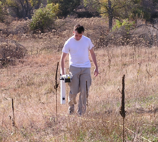
Figure 2.1 Operating the FM36 fluxgate gradiometer.
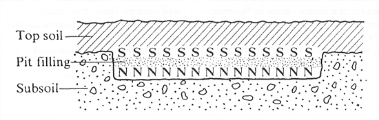
Figure 2.2 Showing the magnetic properties of shallow ditches (Clark 1990).

Figure 2.3 Operating the RM-15 resistance meter.
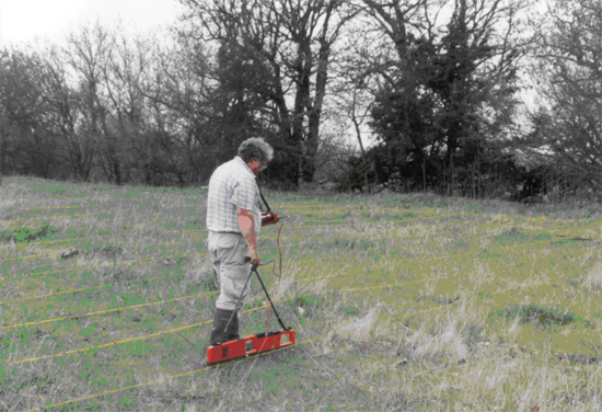
Figure 2.4 Operating the EM38 electromagnetic conductivity meter.
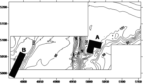
Figure 2.5 Depicting the locations of the initial survey of the Beaver Crossing Site. (0.5 m contour interval)

Figure 2.6 Depicting the locations of the metal diction lines. (0.5 m contour interval)
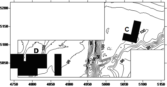
Figure 2.7 Depicting the locations of the second geophysical surveys. (0.5 m contour interval)
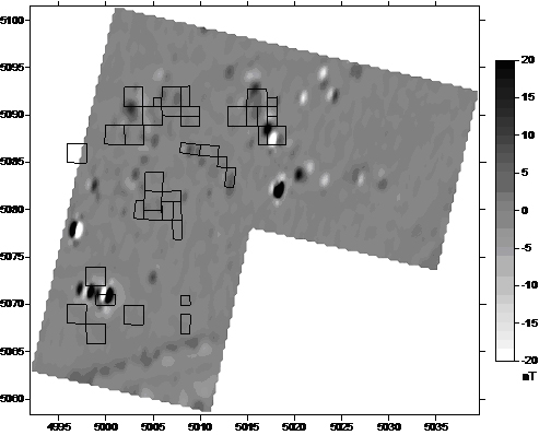
Figure 2.8 Results from the magnetic gradient survey at location A overlaid with the test unit locations.
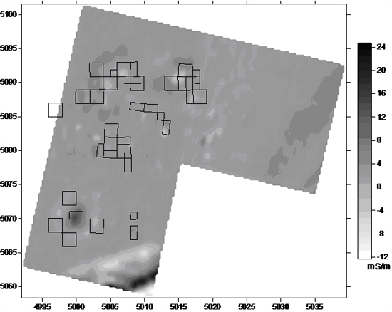
Figure 2.9 Results from the conductivity survey at location A overlaid with the test unit locations.
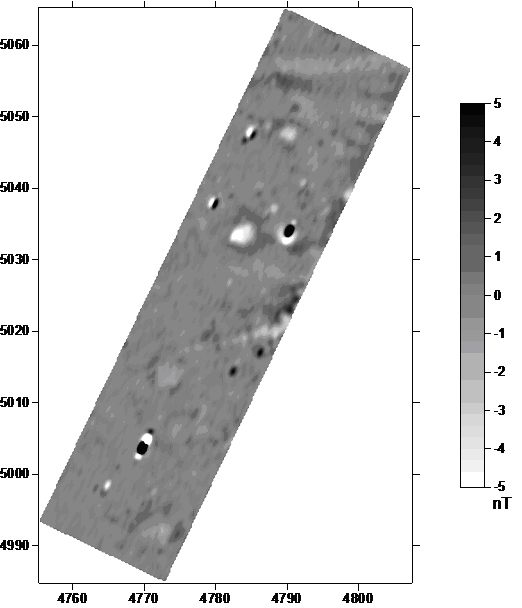
Figure 2.10 Results from the magnetic gradient survey at location B.

Figure 2.11 Results from the conductivity survey at location B
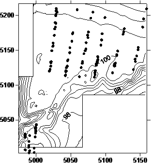
Figure 2.12 Results from the metal detector survey on the east side of the site.
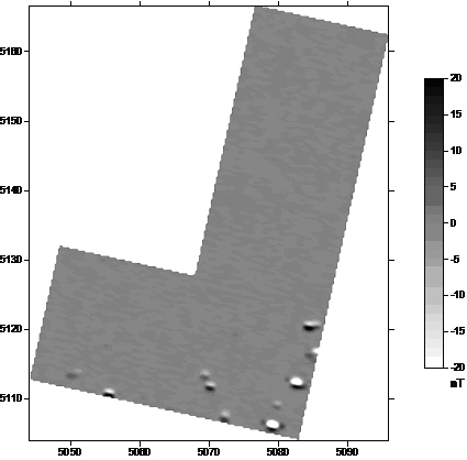
Figure 2.13 Results from the magnetic gradient survey at location C.

Figure 2.14 Results from the magnetic gradient survey at location D.
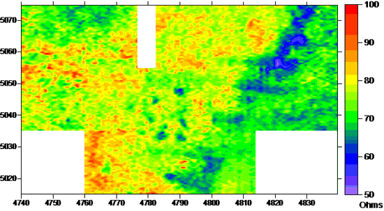
Figure 2.15 Results from the resistance survey at location D.
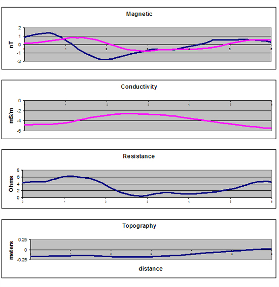
Figure 2.16 Individual profile lines of the trail at areas with visible slope. The initial survey is shown in pink and the second survey is shown in blue.
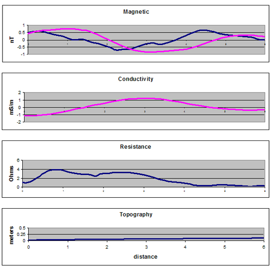
Figure 2.17 Individual profile lines of the trail at areas with no change in topography. The initial survey is shown in pink and the second survey is shown in blue.
Data Recovery Plan for the Beaver Creek Trail Crossing Site, (25SW49) Seward County, Nebraska
By Elizabeth Spott
Site Description
The site is currently owned by Richard Pariset, a local farmer and rancher. For as long as the land has been in his possession, it has served as cow and horse pasture. There is approximately one half mile of wagon ruts visible on both sides of the crossing, which are part of the Nebraska City Cut-off. There are also numerous depressions on both sides of the crossing in the vicinity of the trail remnants. As was mentioned in the Historical Research section, there is a lot of documentation about the location. This information, tied with aerial photos, indicate that this is indeed the location of the original Beaver Crossing.
Due to the lack of till agriculture the site has been preserved quite well. However, a lack of surface artifacts indicates that some soil deposition has taken place since the site was vacated, the extent of which is not known.
Excavation Techniques
The site was originally located in 2004 by Gayle Carlson, Paul Demers, and John Swigart. The site and associated trail ruts were mapped using GPS and entered into the Nebraska State Historical Society GIS database by Swigart. In April and May 2005, the site was surveyed several times by Dr. Demers and Nolan Johnson and Elizabeth Spott, both University of Nebraska–Lincoln graduate students, and others. The survey area included the east and west side of the creek. Also, the creek bed was followed downstream from the site for some distance to determine if artifacts from the site had been or were being washed into the creek. Pedestrian survey was conducted at various intervals, but did not locate any surface artifacts. The goal of the excavation was to determine the location and dimensions of any structures. A decision was made to concentrate efforts on the east side of the creek for several reasons. First, the logistics of moving equipment to and from the west side of the creek was difficult as the water level was very high early in the season and driving to the west side was inefficient due to time. Second, as the excavation was part of the UNL field school, it was determined that teaching would be more effective if all the students and instructors were together. Third, the east side of the creek had topographic features that were interpreted as cultural. These were a large rectangular mound and a circular depression. However, topographic features on the west side of the creek were limited to trail ruts and no evidence of a structure was visible. The first test units were placed adjacent to the mound and depression on the east side of the creek.
The excavation lasted for eight weeks and during that time a total of 41 test units were dug. Seventeen of these units were 2 m by 2m, six were 1 m by 1 m, and 18 were 1 m by 2 m. Of these, only two units, 16 and 17, were placed on the west side of the creek. These were both 2 m by 2m. On the east side of the creek a total of 110 square feet of the site was exposed. Figure 2.18 demonstrates the layout of the test units at the site. The units were dug in 10 cm levels, with each level of each test unit being given a specific provenience number. The units were excavated to varying depths, but all were stopped at the level of sterile yellow clay 4/4 10YR. All of the dirt excavated was dry-screened through ¼" mesh with the exception of samples being taken for flotation. Artifacts were collected and grouped by provenience, and stored temporally for cataloguing and curation.
Artifact Cataloguing and Curation
Artifact washing, sorting, and identification were completed by the Research Methods class at UNL under the supervision of Dr. Demers during the fall of 2005. Artifacts were sorted by provenience, which is a specific test unit and level identifier, and material type, and then stored according to provenience number. Artifacts were catalogued according to specific conventions created for the site by Dr. Demers. First step of cataloguing was identification by material type. These included ceramic, metal, glass, bone, wood, lithic, and miscellaneous. Second, artifacts were placed according to identifiable groups, i.e. nails, whiteware, buttons, etc. Third, groups or individual artifacts were described. The collection is currently being stored at the historical archaeology laboratory at UNL.
References
Aitken, M. J.
1974 Physics and Archaeology. 2nd ed. Oxford University Press, London. Originally published 1961, Interscience Publishers Inc., New York.
Beaver Crossing Centennial Committee
1975 History of Beaver Crossing 1875–1975. Beaver Crossing Centennial Committee, Beaver Crossing, Nebraska.
Beaver Crossing Committee
1932 Community History of Beaver Crossing. Beaver Crossing Committee, Beaver Crossing, Nebraska.
Bevan, B. W.
1998 Geophysical Exploration for Archaeology: An Introduction to Geophysical Exploration. Midwest Archaeological Center, Special Report No. 1.
Clark, A.
1990 Seeing Beneath the Soil: Prospection Methods in Archaeology. 2nd ed. Batsford, London.
Clay, B.
2001 Complementary Geophysical Survey Techniques: Why Two Ways Are Always Better Than One. Southeastern Archaeology 20(1):31–43.
De Vore, S. L.
1996 Magnetic Survey of Camp Lewis, Pecos National Historic Park, San Miguel County, New Mexico. Prepared for Anthropology Program, Intermountain Cultural Resource Center, Intermountain Field Area, National Park Service, Santa Fe, New Mexico.
2005 Geophysical Investigations of Selected Areas within the Beaver Crossing Site (25SW49), Seward County, Nebraska. Midwest Archeological Center, National Park Service, Lincoln, Nebraska.
Gaffney, C. a. J. G.
1991 The Use of Geophysical Techniques in Archaeological Evaluations. Submitted to Institute of Field Archaeologists. Technical Paper 9.
Geonics
1992 EM38 Ground Conductivity Meter Operating Manual for EM38 Models with Digital Readout. Geonics Limited, Mississauga, Ontario, Canada.
1998 DL720/38 Data Logging System Operating Instructions for EM38 Ground Conductivity Meter with Polycorder Series 720, Version 3.40. Geonics Limited, Mississauga, Ontario, Canada.
2002 DAT38W Version 1.10 Computer Program Manual (Survey Data Reduction Manual). Geonics Limited, Mississauga, Ontario, Canada.
Geoscan Research
1987 Fluxgate Gradiometer FM9 FM18 FM36 Instruction Manual, Version 1.0. Geoscan Research, Bradford, England.
2001 Geoplot Version 3.00 for Windows Instruction Manual, Version 1.6. Geoscan Research, Bradford, England.
Golden Software
2002 Surfer 8 User's Guide: Gontouring and 3D Surface Mapping for Scientists and Engineers. Golden Software, Golden, Colorado.
Kvamme, K. L.
2001 Current Practices in Archaeogeophysics. In Earth Sciences and Archaeology, edited by P. Goldberg, V. T. Holiday and C. R. Ferring, pp. 353-384. Kluwer Academic/Plenum Publishers, New York.
2001 Final Report of Geophysical Investigations Conducted at the Menoken Village State Historic Site (32BL2), 1997-1999. ArcheoImaging Lab, Department of Anthropology and Center for Advanced Spatial Technologies, University of Arkansas, Fayetteville.
Milsom, J.
2003 Field Geophysics. 3rd ed. The Geological Field Guide Series. John Wiley & Sons Ltd., England.
Smith, Wm. W.
1937 Early Days in Seward County Nebraska. Wm. H. Smith, Seward, Nebraska.
Waterman, John H.
1927 General History of Seward County Nebraska. Beaver Crossing, Nebraska.
Weymouth, J. W.
1986 Geophysical Methods of Archaeological Site Surveying. Advances in Archaeological Method and Theory 9:311–395.
Wynn, J. C.
1986 Archaeological Prospection: An Introduction to the Special Issue. Geophysics 51(3):533–537.
1986 A Review of Geophysical Methods Used in Archaeology. Geoarchaeology: An International Journal 1 (3):245–257.